Graphing Namebench Spreadsheet Data with R

In the previous post, I described the process of benchmarking domain name servers for a website domain with a modified version of Namebench. Namebench generates graphs using the Google chart API. This left me wanting a little more therefore decided to explore the data using the R Project. This post makes the assumption you are using our data set in order to follow along or else YMMV.

First, remove trailing commas from each row:

$ sed 's/,[[:space:]]*$//' namebench_2015-07-14_1952.csv > data.csv

Next, we read in the data from the CSV file into the R buffer assuming you are already in the R console:

> data <- read.table(file="data.csv",header=TRUE,sep=",",row.names=NULL)

If you get errors about a line not having 9 elements, you likely had timeouts in your DNS queries. You can either re-run the test until you do not experience any timeouts or remove the Timeout error message lines. Something like grep -v Timeout data.csv >a.out and copy back to data.csv or whatever filename you would like to work with.

As an aside, we can also export our data back out:

> write.table(data, 'a.txt', col.names=NA)

Which results in:

"" "IP" "Name" "Test_Num" "Record" "Record_Type" "Duration" "TTL" "Answer_Count" "Response"
"1" "2600:3c01::a" "Linode 2 IPv6" 0 "www.rsreese.com." "A" 76.2228965759277 86400 1 "74.207.234.79"
"2" "2600:3c01::a" "Linode 2 IPv6" 0 "www.rsreese.com." "A" 73.7550258636475 86400 1 "74.207.234.79"
"3" "2600:3c01::a" "Linode 2 IPv6" 0 "www.rsreese.com." "A" 73.4801292419434 86400 1 "74.207.234.79"
"4" "2600:3c01::a" "Linode 2 IPv6" 0 "www.rsreese.com." "A" 76.7168998718262 86400 1 "74.207.234.79"
"5" "2600:3c01::a" "Linode 2 IPv6" 0 "www.rsreese.com." "A" 73.2970237731934 86400 1 "74.207.234.79"
"6" "2600:3c01::a" "Linode 2 IPv6" 0 "www.rsreese.com." "A" 73.3959674835205 86400 1 "74.207.234.79"
"7" "2600:3c01::a" "Linode 2 IPv6" 0 "www.rsreese.com." "A" 72.7560520172119 86400 1 "74.207.234.79"
"8" "2600:3c01::a" "Linode 2 IPv6" 0 "www.rsreese.com." "A" 76.8599510192871 86400 1 "74.207.234.79"
"9" "2600:3c01::a" "Linode 2 IPv6" 0 "www.rsreese.com." "A" 72.8960037231445 86400 1 "74.207.234.79"
"10" "2600:3c01::a" "Linode 2 IPv6" 0 "www.rsreese.com." "A" 74.0060806274414 86400 1 "74.207.234.79"
--snip--

Now that R has our data, we can take a quick look to ensure the columns make sense:

> options(width=150)
> head(data,n=10)
> head(data,n=10)
             IP          Name Test_Num           Record Record_Type Duration   TTL Answer_Count      Response
1  2600:3c01::a Linode 2 IPv6        0 www.rsreese.com.           A 76.22290 86400            1 74.207.234.79
2  2600:3c01::a Linode 2 IPv6        0 www.rsreese.com.           A 73.75503 86400            1 74.207.234.79
3  2600:3c01::a Linode 2 IPv6        0 www.rsreese.com.           A 73.48013 86400            1 74.207.234.79
4  2600:3c01::a Linode 2 IPv6        0 www.rsreese.com.           A 76.71690 86400            1 74.207.234.79
5  2600:3c01::a Linode 2 IPv6        0 www.rsreese.com.           A 73.29702 86400            1 74.207.234.79
6  2600:3c01::a Linode 2 IPv6        0 www.rsreese.com.           A 73.39597 86400            1 74.207.234.79
7  2600:3c01::a Linode 2 IPv6        0 www.rsreese.com.           A 72.75605 86400            1 74.207.234.79
8  2600:3c01::a Linode 2 IPv6        0 www.rsreese.com.           A 76.85995 86400            1 74.207.234.79
9  2600:3c01::a Linode 2 IPv6        0 www.rsreese.com.           A 72.89600 86400            1 74.207.234.79
10 2600:3c01::a Linode 2 IPv6        0 www.rsreese.com.           A 74.00608 86400            1 74.207.234.79
> summary(data$Duration)
   Min. 1st Qu.  Median    Mean 3rd Qu.    Max. 
  1.455   2.582   3.836  24.430  47.640 780.500

We can create an aggregated table of the data based on mean values:

> aggregate(data$Duration, by=list(data$Name), FUN=mean)
         Group.1         x
1        CF Erin  3.752344
2         CF Ram  6.141772
3           HE 1  2.563629
4           HE 2  2.494576
5      HE 2 IPv6  2.677688
6           HE 3  5.510935
7      HE 3 IPv6  3.057263
8           HE 4  2.982669
9      HE 4 IPv6  2.626012
10          HE 5  2.642891
11     HE 5 IPv6  2.736038
12      Linode 1 49.536158
13 Linode 1 IPv6 48.098648
14      Linode 2 75.840130
15 Linode 2 IPv6 76.885061
16      Linode 3 25.727819
17 Linode 3 IPv6 26.703984
18      Linode 4  8.020208
19 Linode 4 IPv6  7.908908
20      Linode 5 82.185041
21 Linode 5 IPv6 76.434550

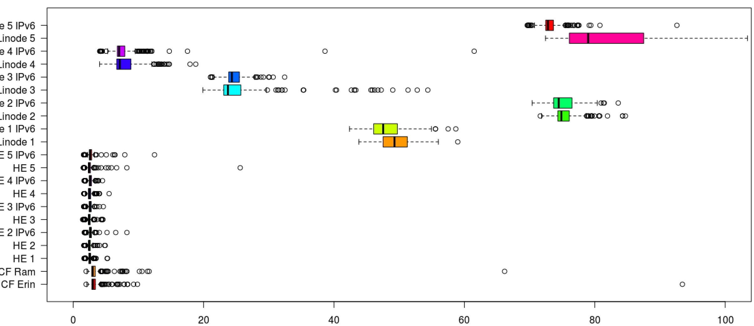
Lets see how a boxplot looks. The graph is representative of the third command listed here, others are for reference/tinkering:

> plot(data$Duration ~ data$Name, horizontal=TRUE, par(las=1))
> boxplot(data$Duration ~ data$Name, horizontal=TRUE, par(las=1), col=rainbow(10))
> boxplot(data$Duration ~ data$Name, ylim=c(0,100), horizontal=TRUE, par(las=1), col=rainbow(10))

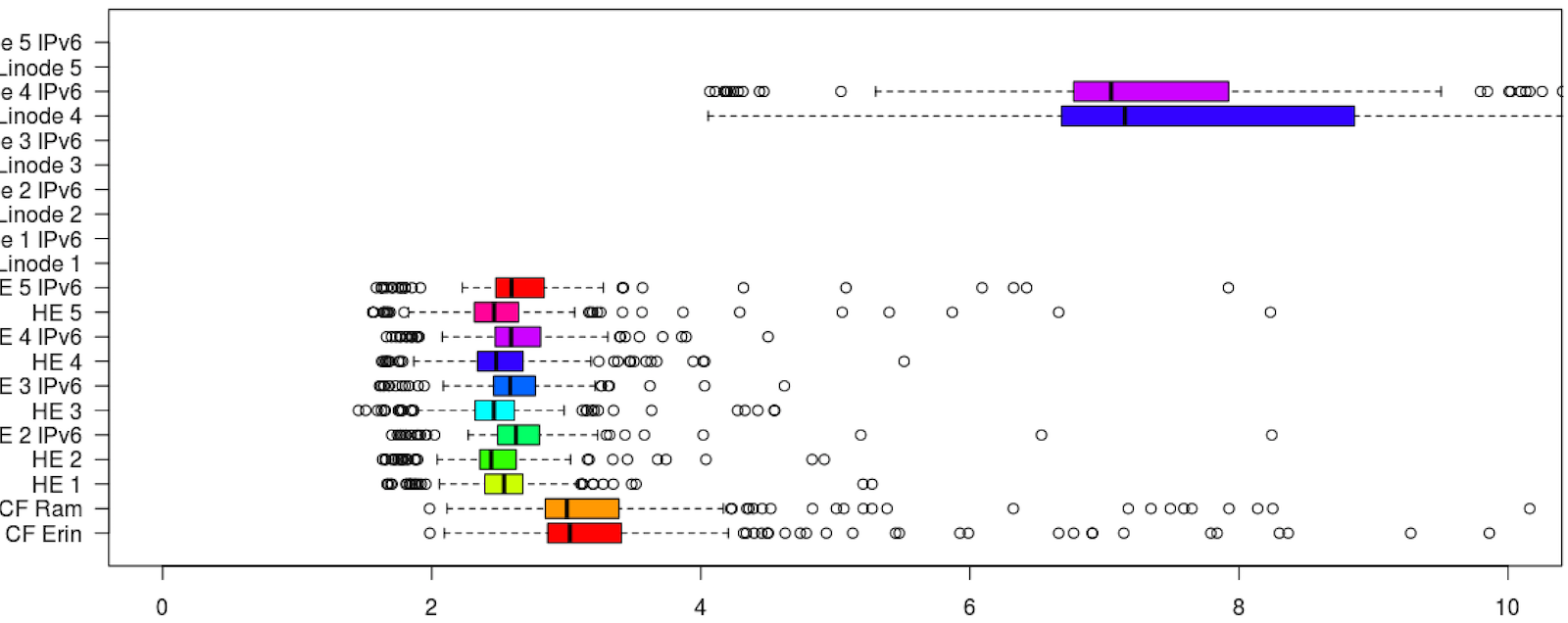
If we zoom in a little more, the distribution of the more responsive name servers becomes apparent. I believe this graph is the best representation of the fastest name servers in the dataset:

> boxplot(data$Duration ~ data$Name, ylim=c(0,10), horizontal=TRUE, par(las=1), col=rainbow(10))

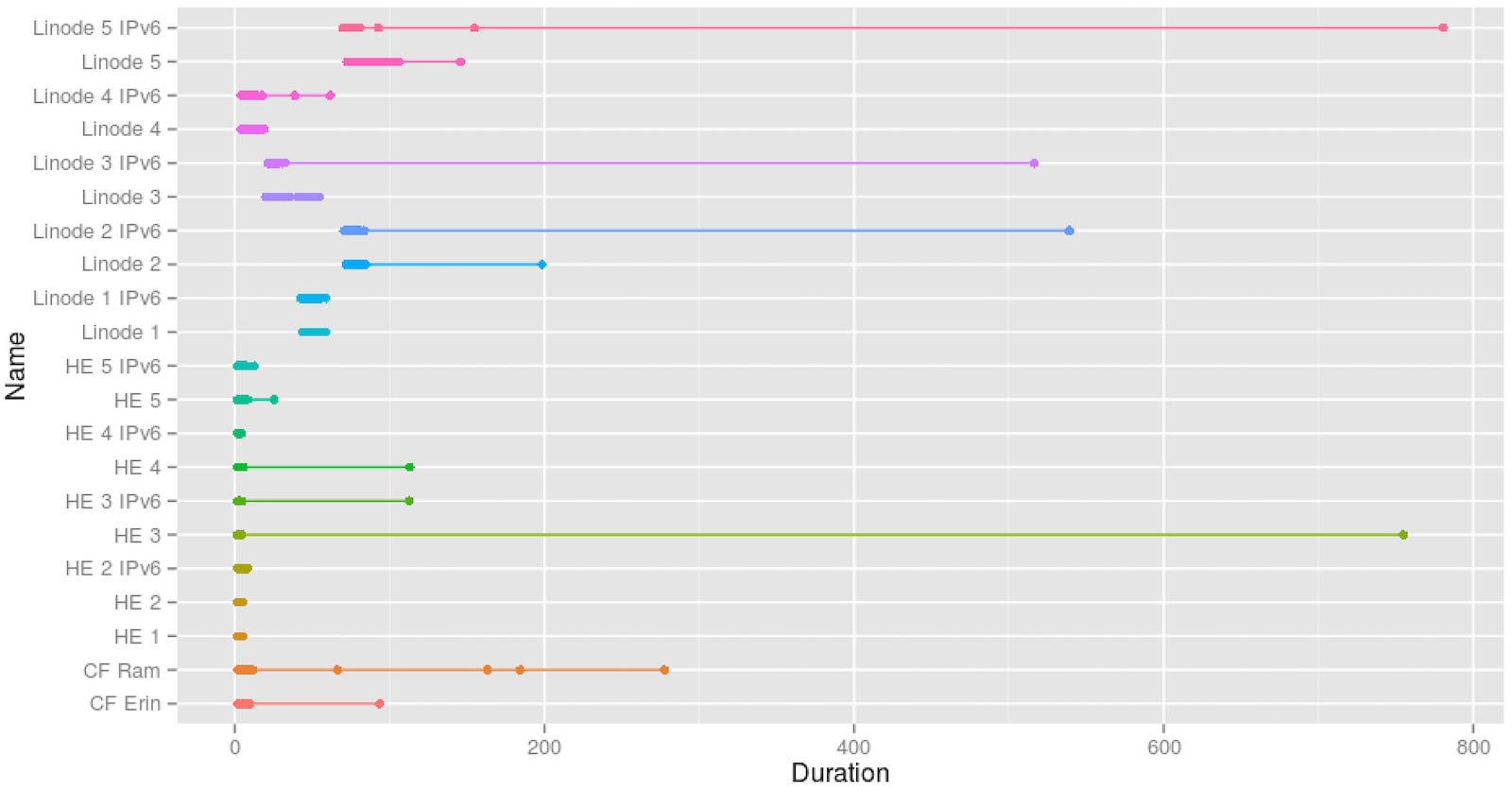
Alternatively, we can plot using ggplot2 if available:

> library(ggplot2)
> ggplot(data=data, aes(x=Duration, y=Name, group=Name, colour=Name)) + geom_line() + geom_point()

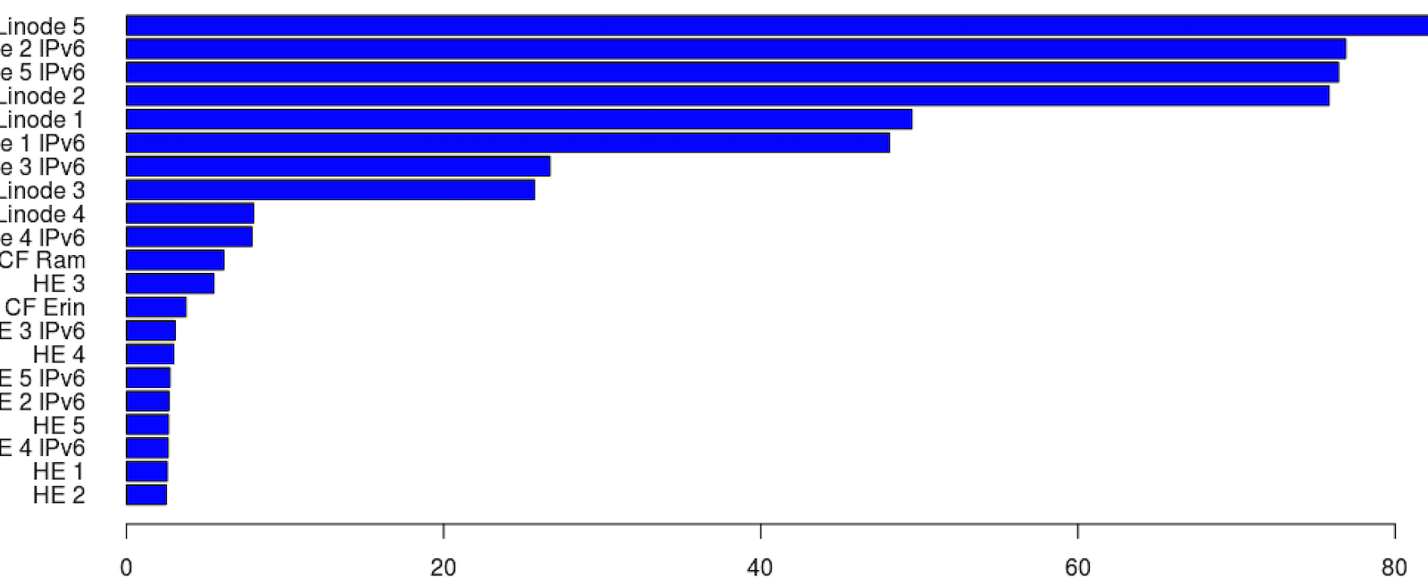
Display horizontal bar graph. I did not do a great job with the axis labels here but you get the idea:

> agg <- aggregate(data$Duration, by=list(data$Name), FUN=mean)
> sorted <- agg[with(agg, order(x)), ]
> mymat <- t(sorted[-1])
> colnames(mymat) <- sorted[, 1]
> barplot(mymat, horiz=TRUE, col=c("blue"), las=1)

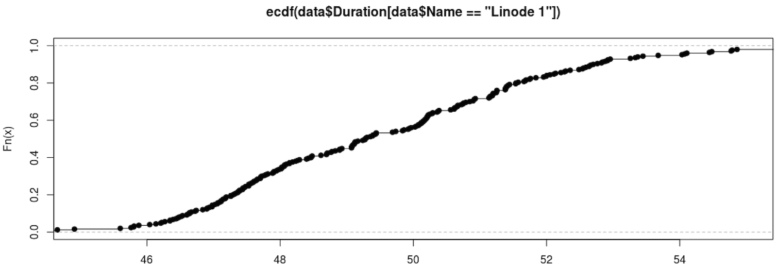
Finally, we will graph a group of values from the set and display them. We also limit the range so the graph is readable:

> plot(ecdf(data$Duration[data$Name=="Linode 1"]), xlim=c(45,55), ylim=c(0,1))

Please leave any questions you have regarding this post below.

Stephen Reese

Graphing Namebench Spreadsheet Data with R

Comments